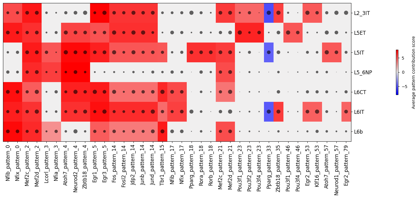
Enhancer code analysis#
In this notebook we will go over how to obtain cell type characteristic sequence patterns from CREsted models, or any other model, using CREsted functionality and the extra packages from crested[motif]: tfmodisco-lite and memesuite-lite.
Obtaining contribution scores per model class and running tfmodisco-lite#
Before we can do any analysis, we need to calculate the contribution scores for cell type-specific regions. These regions hold the most sequence information relevant for cell type identity. From those, we can run tfmodisco-lite.
import anndata as ad
import pandas as pd
import matplotlib.pyplot as plt
import matplotlib.colors as mcolors
import crested
import keras
import pickle
Load data and CREsted model#
We’ll load the dataset and model from the the introduction notebook:
# Set the genome
genome = crested.Genome(
    os.path.join(data_dir, "mm10/mm10.fa"),
    os.path.join(data_dir, "mm10/mm10.chrom.sizes")
)
crested.register_genome(genome)  # Register the genome so that it's automatically used in every function
2026-06-17T15:45:50.909409+0200 INFO Genome mm10 registered.
# Read in the anndata
adata = ad.read_h5ad(os.path.join(data_dir, "mouse_cortex.h5ad"))
# Load a trained model
model_path = "mouse_biccn/finetuned_model/checkpoints/02.keras" # change to your model path
model = crested.utils.load_model(model_path)
Select the most informative regions per cell type#
To obtain cell type-characteristic patterns, we need to calculate contribution scores on highly specific regions. For this purpose, we’ve included a preprocessing function crested.pp.sort_and_filter_regions_on_specificity() to keep the top k most specific regions per cell type that you can use to filter your data before running modisco.
There are three options to select the top regions: either purely based on peak height, purely based on predictions, or on their combination. Here we show how to use the combination of both (which we recommend, see Johansen & Kempynck et al., 2025).
# Store predictions for all our regions in the anndata object
predictions = crested.tl.predict(adata, model)
adata.layers["biccn_model"] = predictions.T
  12/4274 ━━━━━━━━━━━━━━━━━━━━ 1:08 16ms/step
4270/4274 ━━━━━━━━━━━━━━━━━━━━ 0s 16ms/step
4274/4274 ━━━━━━━━━━━━━━━━━━━━ 105s 19ms/step
# Calculate the average of the ground truth and predictions
adata.layers['combined'] = (adata.X + adata.layers["biccn_model"])/2
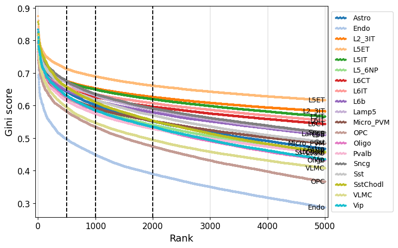
We can use crested.pl.qc.sort_and_filter_cutoff() to look at the gini score distributions for the different regions per class.
Here, we take the top 2000 most specific regions, but top 500 or 1000 regions would give similar results.
%matplotlib inline
crested.pl.qc.sort_and_filter_cutoff(adata, model_name="combined", cutoffs=[500, 1000, 2000], max_k=5000)
2026-03-26T14:55:04.575502+0100 INFO Lazily importing module crested.pl. This could take a second...
# Filter most informative regions per class
top_k = 2000
adata_filtered = crested.pp.sort_and_filter_regions_on_specificity(adata, model_name="combined", top_k=top_k, method="gini", inplace=False)
adata_filtered
2026-03-26T14:55:17.767796+0100 INFO After sorting and filtering, kept 38000 regions.
AnnData object with n_obs × n_vars = 19 × 38000
    obs: 'file_path'
    var: 'chr', 'start', 'end', 'split', 'Class name', 'rank', 'gini_score'
    obsm: 'weights'
    layers: 'DeepBICCN2', 'DeepBICCN2_base', 'gReLU_22M', 'gReLU_6M', 'biccn_model', 'combined'
adata_filtered.var
| chr | start | end | split | Class name | rank | gini_score | |
|---|---|---|---|---|---|---|---|
| region | |||||||
| chr10:45499432-45501546 | chr10 | 45499432 | 45501546 | val | Astro | 1 | 0.827100 |
| chr2:65274604-65276718 | chr2 | 65274604 | 65276718 | train | Astro | 2 | 0.826102 |
| chrX:23135863-23137977 | chrX | 23135863 | 23137977 | train | Astro | 3 | 0.821430 |
| chr1:161272641-161274755 | chr1 | 161272641 | 161274755 | train | Astro | 4 | 0.816905 |
| chr5:9868290-9870404 | chr5 | 9868290 | 9870404 | train | Astro | 5 | 0.810628 |
| ... | ... | ... | ... | ... | ... | ... | ... |
| chr9:22789193-22791307 | chr9 | 22789193 | 22791307 | test | Vip | 1996 | 0.535163 |
| chr6:14177242-14179356 | chr6 | 14177242 | 14179356 | train | Vip | 1997 | 0.535157 |
| chr7:137374461-137376575 | chr7 | 137374461 | 137376575 | train | Vip | 1998 | 0.535079 |
| chr17:57934356-57936470 | chr17 | 57934356 | 57936470 | train | Vip | 1999 | 0.535075 |
| chr1:184003351-184005465 | chr1 | 184003351 | 184005465 | train | Vip | 2000 | 0.535071 |
38000 rows × 7 columns
Calculating contribution scores per class#
Now you can calculate the contribution scores for all the regions in your filtered AnnData.
By default, the contribution scores are calculated using the expected integrated gradients method, but you can change this to simple integrated gradients to speed up the calculation. We’ve found anecdotally that this has a very minor effect on the quality of the contribution scores, while speeding up the calculation significantly.
crested.tl.contribution_scores_specific(
    input=adata_filtered,
    target_idx=None,  # We calculate for all classes
    model=model,
    output_dir="modisco_results_ft_2000",
    method="integrated_grad"
)
Running tfmodisco-lite#
When this is done, you can run TF-MoDISco-lite on the saved contribution scores to find motifs that are important for the classification/regression task.
You could use the tfmodisco package directly to do this, or you could use the crested.tl.modisco.tfmodisco() function which is essentially a wrapper around the tfmodisco package.
Note that from here on, you can use contribution scores from any model trained in any framework, as this analysis just requires a set of one hot encoded sequences and contribution scores per cell type stored in the same directory.
If you don’t have tomtom available on the command line, set report=False in crested.tl.modisco.tfmodisco(). You won’t get an html report matching the motifs to their closest match in the motif database, but you’ll still get a collection of clustered seqlets for use in the rest of the notebook.
meme_db, motif_to_tf_file = crested.get_motif_db()
# run tfmodisco on the contribution scores
crested.tl.modisco.tfmodisco(
    window=1000,
    output_dir="modisco_results_ft_2000",
    contrib_dir="modisco_results_ft_2000",
    report=False,  # Optional, will match patterns to motif MEME database - deactivate if you don't have TOMTOM read on the command line
    meme_db=meme_db,  # File to MEME database - not needed if not generating reports
    max_seqlets=20000,
)
Analysis of cell-type specific sequence patterns#
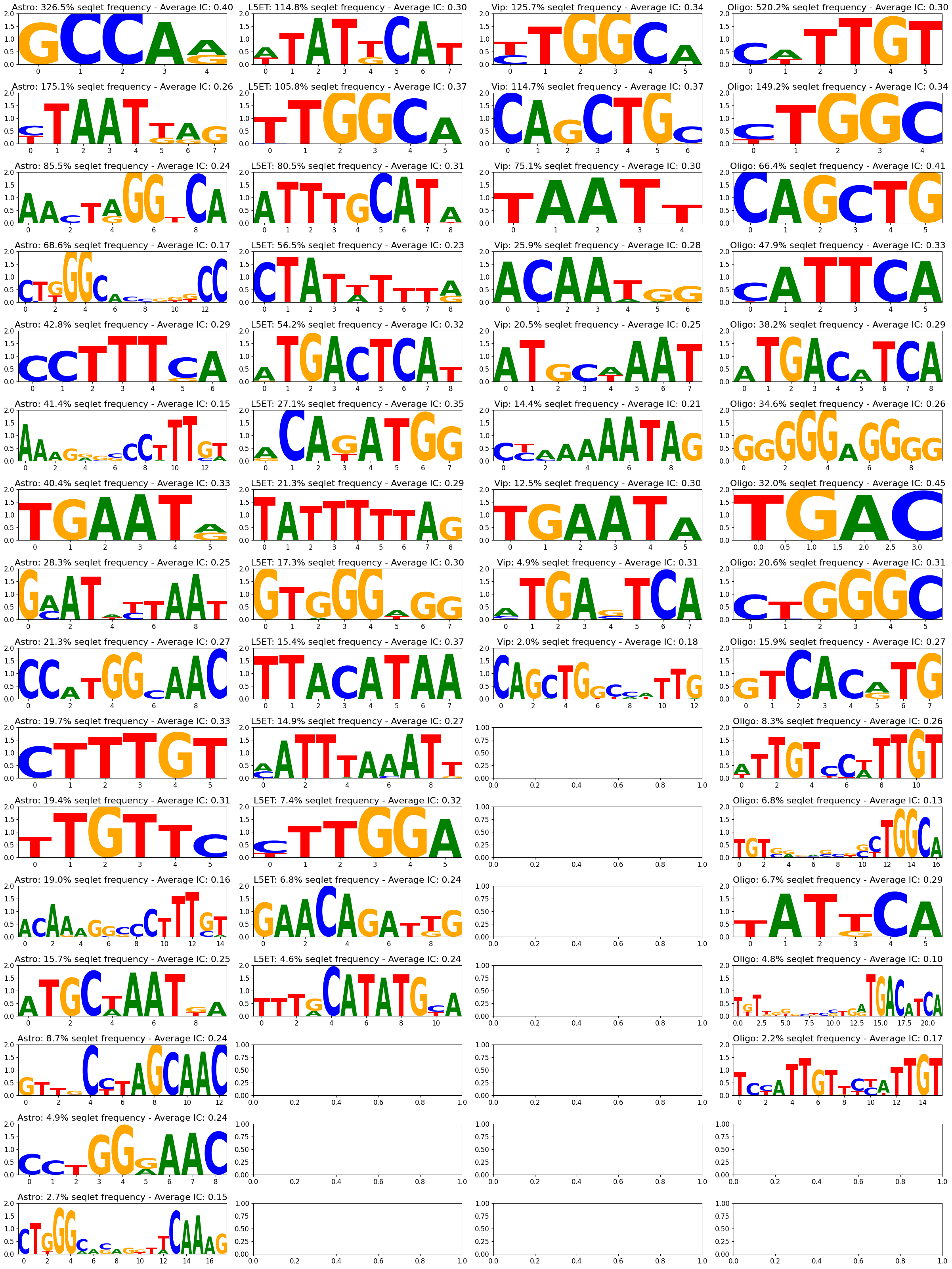
Once you have obtained your modisco results, you can plot the the found patterns using the crested.pl.modisco.modisco_results() function.
%matplotlib inline
top_k = 1000
crested.pl.modisco.modisco_results(
    classes=["Astro", "L5ET", "Vip", "Oligo"],
    contribution="positive",
    contribution_dir="modisco_results_ft_2000",
    num_seq=top_k,
    y_max=0.15,
    viz="pwm",
)  # You can also visualize in 'pwm' format
2026-06-17T15:45:58.619662+0200 INFO Lazily importing module crested.pl. This could take a second...
2026-06-17T15:45:58.935201+0200 INFO Starting genomic contributions plot for classes: ['Astro', 'L5ET', 'Vip', 'Oligo']
Matching patterns across cell types#
Since we have calculated per cell type the patterns independently of each other, we do not know quantitatively how and if they overlap. It can be interesting to get an overview of which patterns are found across multiple cell types, how important they are, and if there are unique patterns only found in a small selection of classes. Therefore, we have made a pattern clustering algorithm, which starts from the results of tfmodisco-lite, and returns a pattern matrix, which contains the importance of the clustered patterns per cell type, and a pattern dictionary, describing all clustered patterns.
First, we’ll obtain the modisco files per class by using crested.tl.modisco.match_h5_files_to_classes() using our selected classes.
# First we obtain the resulting modisco files per class
matched_files = crested.tl.modisco.match_h5_files_to_classes(
    contribution_dir="modisco_results_ft_2000", classes=list(adata.obs_names)
)
A quick pairwise comparison#
Before we do any pattern clustering, we can check for each independent pattern how similar it is to all the other patterns using memesuite-lite.
We use crested.tl.modisco.calculate_tomtom_similarity_per_pattern(). This function returns a pairwise similarity matrix of every unique pattern, together with a list of ids and a dictionary containing additional information per pattern.
sim_matrix, pattern_ids, pattern_dict = crested.tl.modisco.calculate_tomtom_similarity_per_pattern(
    matched_files=matched_files, trim_ic_threshold=0.025, verbose=True
)
Reading file modisco_results_ft_2000/Astro_modisco_results.h5
Reading file modisco_results_ft_2000/Endo_modisco_results.h5
Reading file modisco_results_ft_2000/L2_3IT_modisco_results.h5
Reading file modisco_results_ft_2000/L5ET_modisco_results.h5
Reading file modisco_results_ft_2000/L5IT_modisco_results.h5
Reading file modisco_results_ft_2000/L5_6NP_modisco_results.h5
Reading file modisco_results_ft_2000/L6CT_modisco_results.h5
Reading file modisco_results_ft_2000/L6IT_modisco_results.h5
Reading file modisco_results_ft_2000/L6b_modisco_results.h5
Reading file modisco_results_ft_2000/Lamp5_modisco_results.h5
Reading file modisco_results_ft_2000/Micro_PVM_modisco_results.h5
Reading file modisco_results_ft_2000/OPC_modisco_results.h5
Reading file modisco_results_ft_2000/Oligo_modisco_results.h5
Reading file modisco_results_ft_2000/Pvalb_modisco_results.h5
Reading file modisco_results_ft_2000/Sncg_modisco_results.h5
Reading file modisco_results_ft_2000/Sst_modisco_results.h5
Reading file modisco_results_ft_2000/SstChodl_modisco_results.h5
Reading file modisco_results_ft_2000/VLMC_modisco_results.h5
Reading file modisco_results_ft_2000/Vip_modisco_results.h5
Total patterns: 354
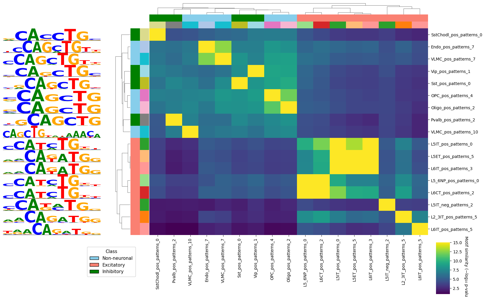
We can now visualize this similarities using crested.pl.modisco.clustermap_tomtom_similarities(). We will subset the often large similarity matrix to a relevant subset. First, we will look at a pattern and find other patterns similar to it in other cell types. We add some additional group labels for visualization purposes.
nn = {"Astro", "Endo", "Micro_PVM", "OPC", "Oligo", "VLMC"}
exc = {"L2_3IT", "L5ET", "L5IT", "L5_6NP", "L6CT", "L6IT", "L6b"}
inh = {"Lamp5", "Pvalb", "Sncg", "Sst", "SstChodl", "Vip"}

groups, groups_2 = [], []
for id in pattern_ids:
    ct = "_".join(id.split("_")[:-3])
    groups.append(
        "Non-neuronal"
        if ct in nn
        else "Excitatory"
        if ct in exc
        else "Inhibitory"
        if ct in inh
        else (_ for _ in ()).throw(ValueError(f"Unknown class: {ct}"))
    )
    groups_2.append(ct)

unique_cats = pd.unique(groups_2)
group_colors_2 = {cat: mcolors.to_hex(plt.get_cmap("tab20", len(unique_cats))(i)) for i, cat in enumerate(unique_cats)}
group_colors = {"Non-neuronal": "skyblue", "Excitatory": "salmon", "Inhibitory": "green"}
%matplotlib inline
crested.pl.modisco.clustermap_tomtom_similarities(
    sim_matrix=sim_matrix,
    ids=pattern_ids,
    pattern_dict=pattern_dict,
    group_info=[(groups, group_colors), (groups_2, group_colors_2)],  # Grouping labels
    query_id="Vip_pos_patterns_1",  # Find patterns similar to this one
    threshold=3,  # TOMTOM similarity threshold, we take the -log10(pval)
    min_seqlets=100,  # Add a minimum amount of seqlets to take the most relevant patterns
)
<seaborn.matrix.ClusterGrid at 0x7f9958764690>
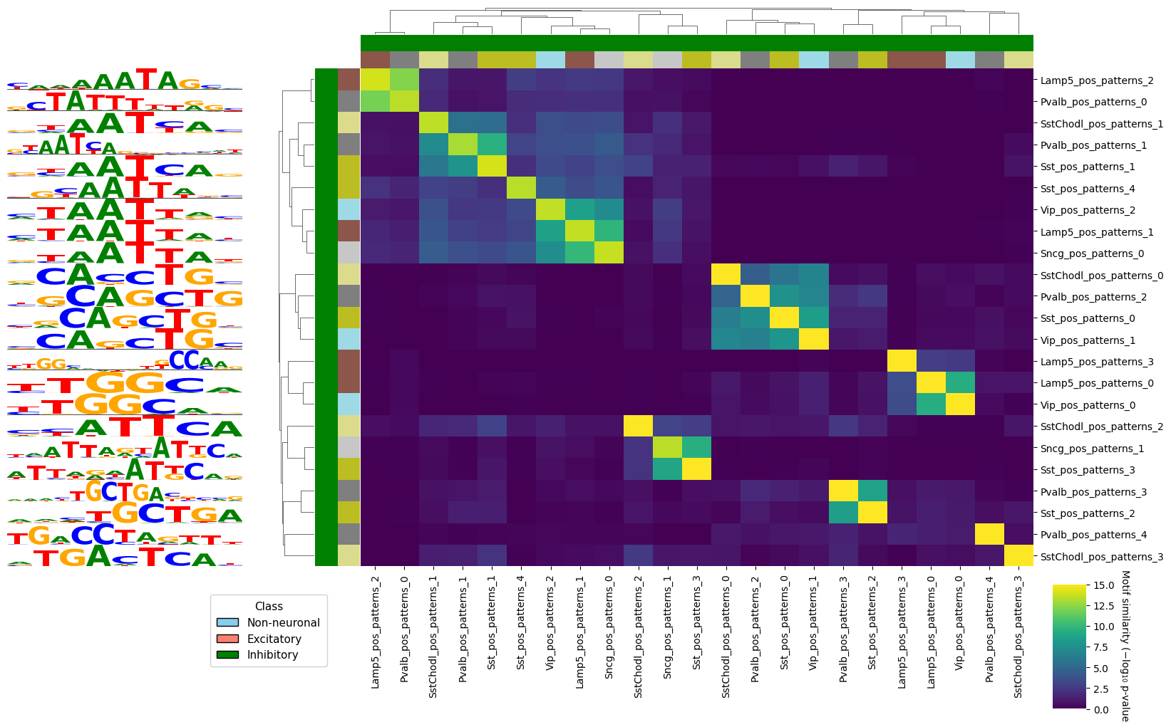
We can also use this to look at all the different patterns in a subset of cell types, and see if we can find interesting groups of similar motifs.
crested.pl.modisco.clustermap_tomtom_similarities(
    sim_matrix=sim_matrix,
    ids=pattern_ids,
    pattern_dict=pattern_dict,
    group_info=[(groups, group_colors), (groups_2, group_colors_2)],  # Grouping labels
    class_names=["Lamp5", "Pvalb", "Sncg", "Sst", "SstChodl", "Vip"],  # Subset of classes to use patterns from
    min_seqlets=300,  # Add a minimum amount of seqlets to take the most relevant patterns
)
<seaborn.matrix.ClusterGrid at 0x7f99585d5350>
Pattern clustering across cell types#
Since many patterns are similar and recur across cell types, we cluster them into groups and compare the importance of each matched motif over all cell types. We cluster all separate patterns with crested.tl.modisco.process_patterns() and summarise them into a pattern matrix with crested.tl.modisco.create_pattern_matrix().
crested.tl.modisco.process_patterns() IC-trims every pattern, computes the full pairwise TOMTOM similarity (-log10(p), via memesuite-lite), turns it into a distance, and runs agglomerative hierarchical clustering (linkage_method="average") cut at sim_threshold — deterministic and order-independent (pass clustering="greedy" for the older order-dependent leader clustering). Each cluster keeps one representative motif (the logo shown, and the PPM later matched to a TF), chosen by representative: "n_seqlets" (default) uses the most-supported instance, "ic_total" the most complete motif, and "ic_mean" the legacy choice that biases toward short motifs. Raise sim_threshold for more, tighter clusters.
# Then we cluster matching patterns, and define a pattern matrix [#classes, #patterns] describing their importance
all_patterns = crested.tl.modisco.process_patterns(
    matched_files,
    sim_threshold=6,             # −log10(p) TOMTOM cut: higher = more, tighter clusters
    trim_ic_threshold=0.03,        # IC flank trimming before similarity
    discard_ic_threshold=0.2,      # drop low-IC single-class clusters
    clustering="agglomerative",    # deterministic, order-independent (previously "greedy")
    linkage_method="average",      # controls chaining better than single linkage
    sort_by="n_seqlets",           # cluster ids ordered by total seqlet support
    representative="n_seqlets",    # cluster's shown/matched motif = most-supported instance
    verbose=True,
)
pattern_matrix = crested.tl.modisco.create_pattern_matrix(
    classes=list(adata.obs_names),
    all_patterns=all_patterns,
    normalize=False,
    pattern_parameter="seqlet_count_log",
)
pattern_matrix.shape
# Optional: save the matched patterns if you want to re-use them later
with open("modisco_results_ft_2000/all_patterns.pkl", 'wb') as f:
    pickle.dump(all_patterns, f)
Now we can plot a clustermap of cell types/classes and patterns, where the classes are clustered
purely on pattern importance with crested.tl.modisco.generate_nucleotide_sequences() and crested.pl.modisco.clustermap()
pat_seqs = crested.tl.modisco.generate_nucleotide_sequences(all_patterns)
crested.pl.modisco.clustermap(
    pattern_matrix,
    list(adata.obs_names),
    width=25,
    height=4.2,
    pat_seqs=pat_seqs,
    grid=True,
    dendrogram_ratio=(0.03, 0.15),
    importance_threshold=4,
)
<seaborn.matrix.ClusterGrid at 0x7f99c4222f10>

If you have the horizontal space for it, you can also add the PWM/contribution logos to the x-axis.
crested.pl.modisco.clustermap_with_pwm_logos(
    pattern_matrix,
    list(adata.obs_names),
    pattern_dict=all_patterns,
    width=50,
    height=4.2,
    grid=True,
    dendrogram_ratio=(0.03, 0.15),
    importance_threshold=4,
    logo_x_multiplier=1,
    logo_height_fraction=0.35,
    logo_y_padding=0.25,
)
<seaborn.matrix.ClusterGrid at 0x7f99d036ad90>

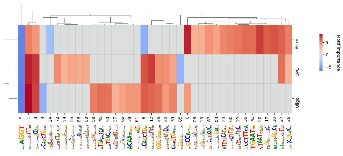
We can also subset to classes we are interested in and want to compare in more detail.
crested.pl.modisco.clustermap_with_pwm_logos(
    pattern_matrix,
    classes=list(adata.obs_names),
    pattern_dict=all_patterns,
    subset=["Astro", "OPC", "Oligo"],
    width=10,
    height=3,
    grid=True,
    logo_height_fraction=0.35,
    logo_y_padding=0.3,
)
<seaborn.matrix.ClusterGrid at 0x7f988bc26450>
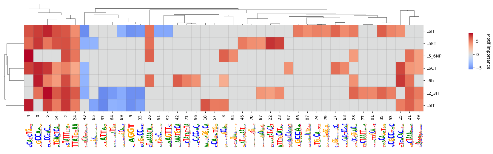
crested.pl.modisco.clustermap_with_pwm_logos(
    pattern_matrix,
    classes=list(adata.obs_names),
    subset=["L2_3IT", "L5ET", "L5IT", "L5_6NP", "L6CT", "L6IT", "L6b"],
    pattern_dict=all_patterns,
    width=15,
    height=3,
    grid=True,
    logo_height_fraction=0.35,
    logo_y_padding=0.3,
    importance_threshold=4,
)
<seaborn.matrix.ClusterGrid at 0x7f98b6348650>
Additional pattern insights#
It’s always interesting to investigate specific patterns that show in the clustermap above. Here there are some example functions with which to do that.
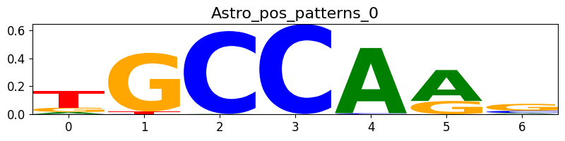
Plotting patterns based on their indices can be done with crested.pl.modisco.selected_instances():
pattern_indices = [0]
crested.pl.modisco.selected_instances(
    all_patterns, pattern_indices
)  # Shows the cluster's representative instance (most seqlets by default; see process_patterns(representative=...))
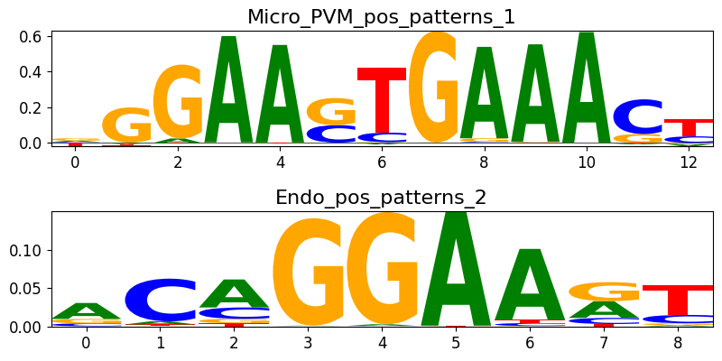
We can also do a check of pattern similarity:
idx1 = 30
idx2 = 34
sim = crested.tl.modisco.pattern_similarity(all_patterns, idx1, idx2)
print("Pattern similarity is " + str(sim))
crested.pl.modisco.selected_instances(all_patterns, [idx1, idx2])
Pattern similarity is 1.3679798404509877
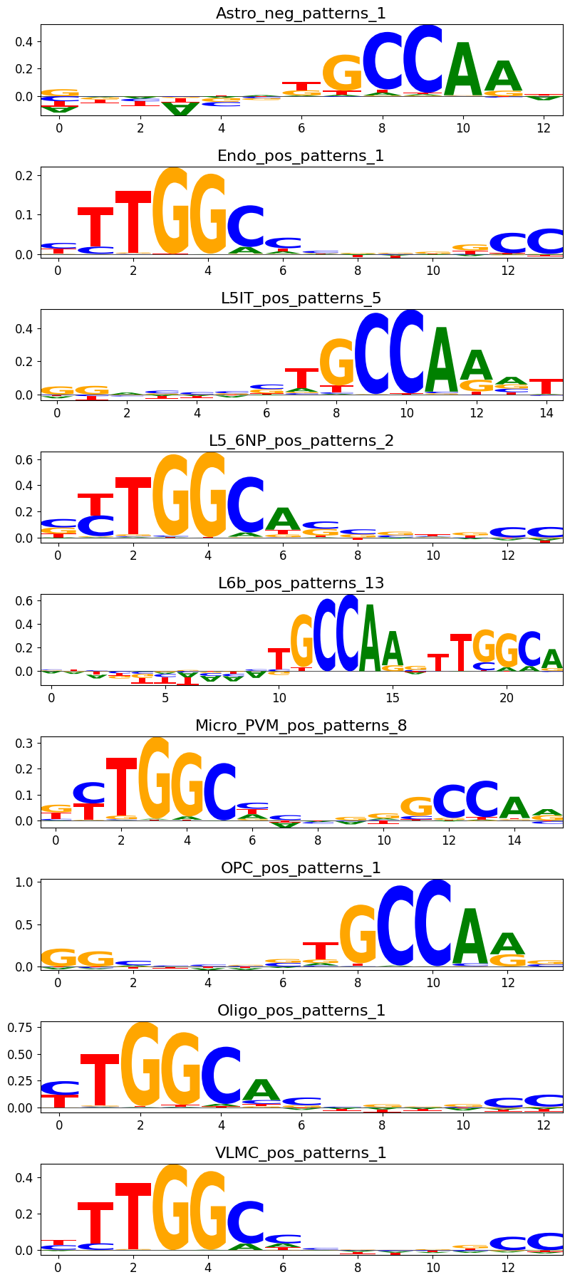
We can plot all the instances of patterns in the same cluster with crested.pl.modisco.class_instances():
crested.pl.modisco.class_instances(all_patterns, 3)
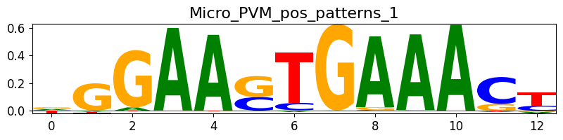
If you want to find out in which pattern cluster a certain pattern is from your modisco results, you can use the crested.tl.modisco.find_pattern() function.
idx = crested.tl.modisco.find_pattern("Micro_PVM_pos_patterns_1", all_patterns)
if idx is not None:
    print("Pattern index is " + str(idx))
    crested.pl.modisco.class_instances(all_patterns, idx, class_representative=True)
Pattern index is 30
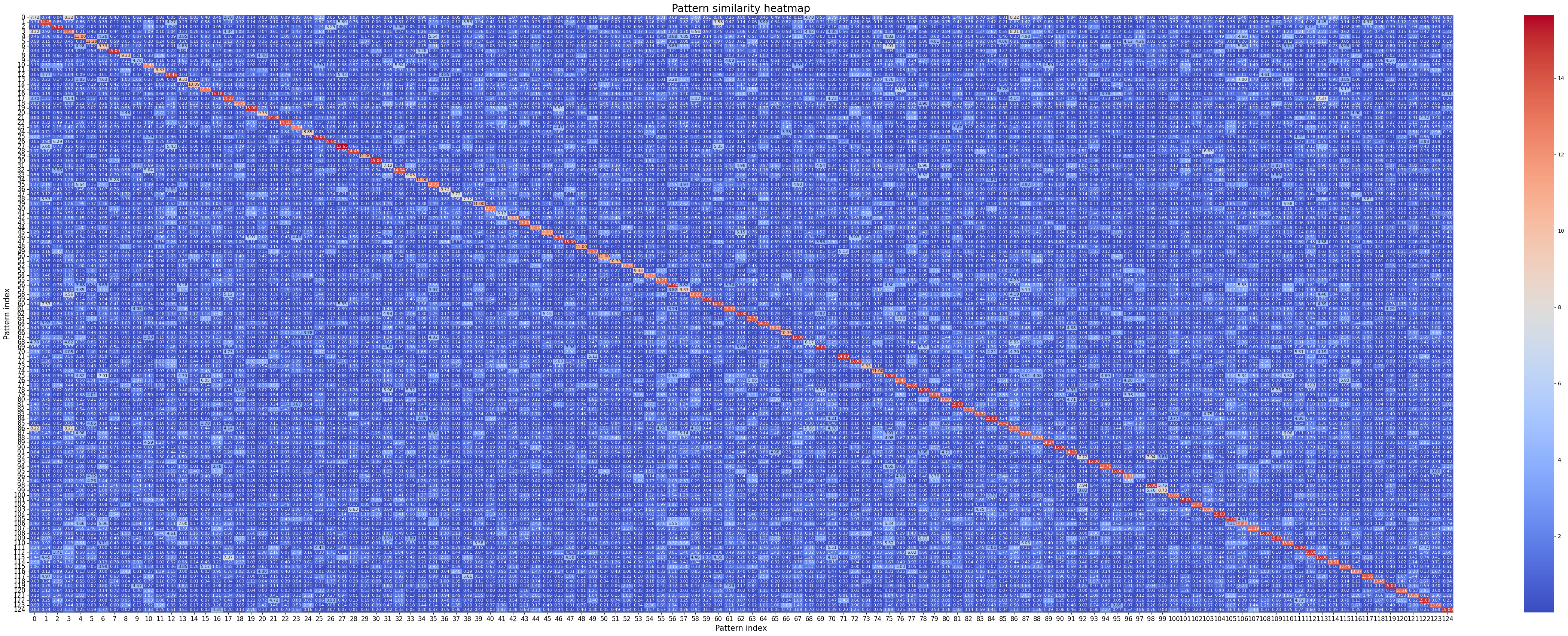
Finally, we can also plot the similarity between all patterns with crested.tl.modisco.calculate_similarity_matrix() and crested.pl.modisco.similarity_heatmap():
sim_matrix, indices = crested.tl.modisco.calculate_similarity_matrix(all_patterns)
crested.pl.modisco.similarity_heatmap(sim_matrix, indices, fig_size=(42, 17))
2026-06-17T15:50:29.534036+0200 WARNING `fig_size` is deprecated since version 1.7.0; please use arguments `width=42, height=17` instead.
Matching patterns to TF candidates from scRNA-seq data [Optional]#
To understand the actual transcription factor (TF) candidates binding to the characteristic patterns/potential binding sites per cell type, we can propose potential candidates through scRNA-seq data and a TF-motif collection file.
This analysis requires that you ran tfmodisco-lite with the report function such that each pattern has potential MEME database hits and that you have multiome data. The names in the motif database should match those in the TF-motif collection file.
meme_db, motif_to_tf_file = crested.get_motif_db()
If you haven’t run this yet and using crested.tl.modisco.tfmodisco did not work due to lack of access to TOMTOM, versions of modiscolite above v2.4.0 also support using memelite with argument ttl=True, meaning you can generate the reports this way:
# If you don't have the patterns loaded, load here
with open('modisco_results_ft_2000/all_patterns.pkl', 'rb') as f:
    all_patterns = pickle.load(f)
Load scRNA-seq data#
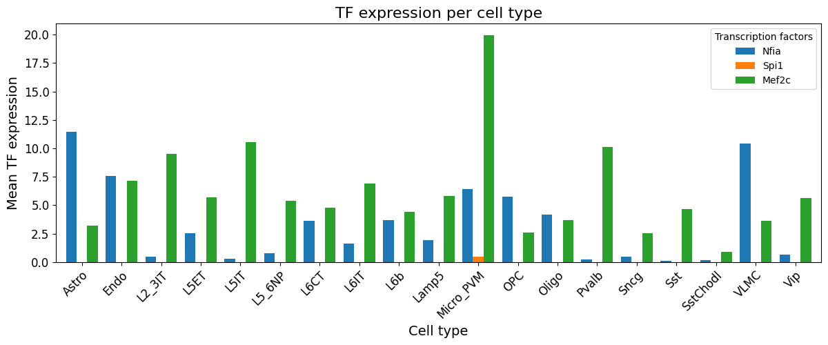
Load scRNA seq data and calculate mean expression per cell type using crested.tl.modisco.calculate_mean_expression_per_cell_type().
file_path = os.path.join(data_dir,"mouse_cortex_scrna.h5ad")  # Locate h5 file containing scRNAseq data, from Zemke et al., 2023, Nature
cell_type_column = "subclass_Bakken_2022"
mean_expression_df = crested.tl.modisco.calculate_mean_expression_per_cell_type(
    file_path, cell_type_column, cpm_normalize=True
)
Please make sure that the classes in the RNA file match those used in CREsted, and rename mean_expression_df’s index if not:
# Rename classes that don't match exactly (due to / being cleaned up to _, etc)
# Here they're in the same (alphabetical) order anyway so we can just zip them
class_mapping = dict(zip(mean_expression_df.index, adata.obs_names, strict=True))
print(class_mapping)

mean_expression_df.index = mean_expression_df.index.map(class_mapping)
{'Astro': 'Astro', 'Endo': 'Endo', 'L2/3 IT': 'L2_3IT', 'L5 ET': 'L5ET', 'L5 IT': 'L5IT', 'L5/6 NP': 'L5_6NP', 'L6 CT': 'L6CT', 'L6 IT': 'L6IT', 'L6b': 'L6b', 'Lamp5': 'Lamp5', 'Micro-PVM': 'Micro_PVM', 'OPC': 'OPC', 'Oligo': 'Oligo', 'Pvalb': 'Pvalb', 'Sncg': 'Sncg', 'Sst': 'Sst', 'Sst Chodl': 'SstChodl', 'VLMC': 'VLMC', 'Vip': 'Vip'}
crested.pl.modisco.tf_expression_per_cell_type(mean_expression_df, ["Nfia", "Spi1", "Mef2c"])
Generating pattern to database motif dictionary#
classes = list(adata.obs_names)
contribution_dir = "modisco_results_ft_2000"
html_paths = crested.tl.modisco.generate_html_paths(all_patterns, classes, contribution_dir)

# p_val threshold to only select significant matches
pattern_match_dict = crested.tl.modisco.find_pattern_matches(
    all_patterns, html_paths, p_val_thr=0.05
)
Loading TF-motif database#
motif_to_tf_df = crested.tl.modisco.read_motif_to_tf_file(motif_to_tf_file)
motif_to_tf_df
| logo | Motif_name | Cluster | Human_Direct_annot | Human_Orthology_annot | Mouse_Direct_annot | Mouse_Orthology_annot | Fly_Direct_annot | Fly_Orthology_annot | Cluster_Human_Direct_annot | Cluster_Human_Orthology_annot | Cluster_Mouse_Direct_annot | Cluster_Mouse_Orthology_annot | Cluster_Fly_Direct_annot | Cluster_Fly_Orthology_annot | |
|---|---|---|---|---|---|---|---|---|---|---|---|---|---|---|---|
| 0 | <img src="https://motifcollections.aertslab.org/v10/logos/bergman__Adf1.png" height="52" alt="bergman__Adf1"></img> | bergman__Adf1 | NaN | NaN | NaN | NaN | NaN | Adf1 | NaN | NaN | NaN | NaN | NaN | NaN | NaN |
| 1 | <img src="https://motifcollections.aertslab.org/v10/logos/bergman__Aef1.png" height="52" alt="bergman__Aef1"></img> | bergman__Aef1 | NaN | NaN | NaN | NaN | NaN | Aef1 | NaN | NaN | NaN | NaN | NaN | NaN | NaN |
| 2 | <img src="https://motifcollections.aertslab.org/v10/logos/bergman__ap.png" height="52" alt="bergman__ap"></img> | bergman__ap | NaN | NaN | NaN | NaN | NaN | ap | NaN | NaN | NaN | NaN | NaN | NaN | NaN |
| 3 | <img src="https://motifcollections.aertslab.org/v10/logos/elemento__ACCTTCA.png" height="52" alt="elemento__ACCTTCA"></img> | elemento__ACCTTCA | NaN | NaN | NaN | NaN | NaN | NaN | NaN | NaN | NaN | NaN | NaN | NaN | NaN |
| 4 | <img src="https://motifcollections.aertslab.org/v10/logos/bergman__bcd.png" height="52" alt="bergman__bcd"></img> | bergman__bcd | NaN | NaN | NaN | NaN | NaN | bcd | NaN | NaN | NaN | NaN | NaN | NaN | NaN |
| ... | ... | ... | ... | ... | ... | ... | ... | ... | ... | ... | ... | ... | ... | ... | ... |
| 17990 | <img src="https://motifcollections.aertslab.org/v10/logos/elemento__CAAGGAG.png" height="52" alt="elemento__CAAGGAG"></img> | elemento__CAAGGAG | 98.3 | NaN | NaN | NaN | NaN | NaN | NaN | NaN | NaN | NaN | NaN | NaN | NaN |
| 17991 | <img src="https://motifcollections.aertslab.org/v10/logos/elemento__TCCTTGC.png" height="52" alt="elemento__TCCTTGC"></img> | elemento__TCCTTGC | 98.3 | NaN | NaN | NaN | NaN | NaN | NaN | NaN | NaN | NaN | NaN | NaN | NaN |
| 17992 | <img src="https://motifcollections.aertslab.org/v10/logos/swissregulon__hs__ZNF274.png" height="52" alt="swissregulon__hs__ZNF274"></img> | swissregulon__hs__ZNF274 | 99.1 | ZNF274 | NaN | NaN | Zfp369, Zfp110 | NaN | NaN | ZNF274 | NaN | NaN | Zfp369, Zfp110 | NaN | NaN |
| 17993 | <img src="https://motifcollections.aertslab.org/v10/logos/swissregulon__sacCer__THI2.png" height="52" alt="swissregulon__sacCer__THI2"></img> | swissregulon__sacCer__THI2 | 99.2 | NaN | NaN | NaN | NaN | NaN | NaN | NaN | NaN | NaN | NaN | NaN | NaN |
| 17994 | <img src="https://motifcollections.aertslab.org/v10/logos/jaspar__MA0407.1.png" height="52" alt="jaspar__MA0407.1"></img> | jaspar__MA0407.1 | 99.2 | NaN | NaN | NaN | NaN | NaN | NaN | NaN | NaN | NaN | NaN | NaN | NaN |
17995 rows × 15 columns
Matching patterns to TF candidates#
We link each pattern cluster to candidate transcription factors and score them per cell type with crested.tl.modisco.create_pattern_tf_dict() and crested.tl.modisco.create_tf_ct_matrix().
crested.tl.modisco.create_pattern_tf_dict() collects, per cluster, the TFs whose database motifs match its representative: a deliberately broad candidate pool. crested.tl.modisco.create_tf_ct_matrix() then uses expression to decide which candidate TF(s) actually explain each pattern (selection="nnls", the default): a pattern is annotated only if a candidate’s expression peaks (zscore_threshold) and tracks the pattern’s importance profile across cell types (correlation_threshold); that importance profile is modelled as a non-negative ridge combination of all the candidates’ expression profiles, so broadly-expressed binders that merely correlate are competed down; and a final expression-relevance gate (rel_keep_frac) keeps only TFs expressed where the pattern fires, dropping barely-expressed paralogs while keeping genuinely co-expressed ones. Pass selection="threshold" for the original per-column correlation/z-score filter.
cols = [
    "Mouse_Direct_annot",
    "Mouse_Orthology_annot",
    "Cluster_Mouse_Direct_annot",
    "Cluster_Mouse_Orthology_annot",
]
pattern_tf_dict, all_tfs = crested.tl.modisco.create_pattern_tf_dict(
    pattern_match_dict, motif_to_tf_df, all_patterns, cols
)
tf_ct_matrix, tf_pattern_annots = crested.tl.modisco.create_tf_ct_matrix(
    pattern_tf_dict,
    all_patterns,
    mean_expression_df,
    classes,
    log_transform=True,
    normalize_pattern_importances=False,
    normalize_gex=True,
    min_tf_gex=0,               # raw-expression floor on the firing cell types
    importance_threshold=4,
    pattern_parameter="seqlet_count_log",
    selection="nnls",              # deconvolution + expression-relevance gate (default)
    nnls_alpha=1.0,                # ridge: spreads weight over collinear paralogs
    nnls_keep_frac=0.2,            # keep TFs with weight ≥ 0.2·max within a pattern
    rel_keep_frac=0.1,             # keep TFs actually expressed where the pattern fires (1+ paralogs)
    zscore_threshold=1.5,          # pattern gate
    correlation_threshold=0.45,    # pattern gate
    verbose=True,
)
create_tf_ct_matrix - TF-pattern candidate filtering:
  candidates (TF-motif pairs) : 1074  (skipped 221: TF absent from expression table)
  after gex/importance gate   :  678  (dropped 396; min_tf_gex=0 on input expr, importance_threshold=4)
      input expr on firing CTs (peak/candidate): p10=0.000501 p50=0.0686 p90=0.994  -> calibrate min_tf_gex here
  after nnls regression       :  146  (dropped 532; alpha=1.0, keep_frac=0.2)
  after relevance gate        :  105  (dropped 41; rel_keep_frac=0.1)
  -> kept 105 TF-pattern columns
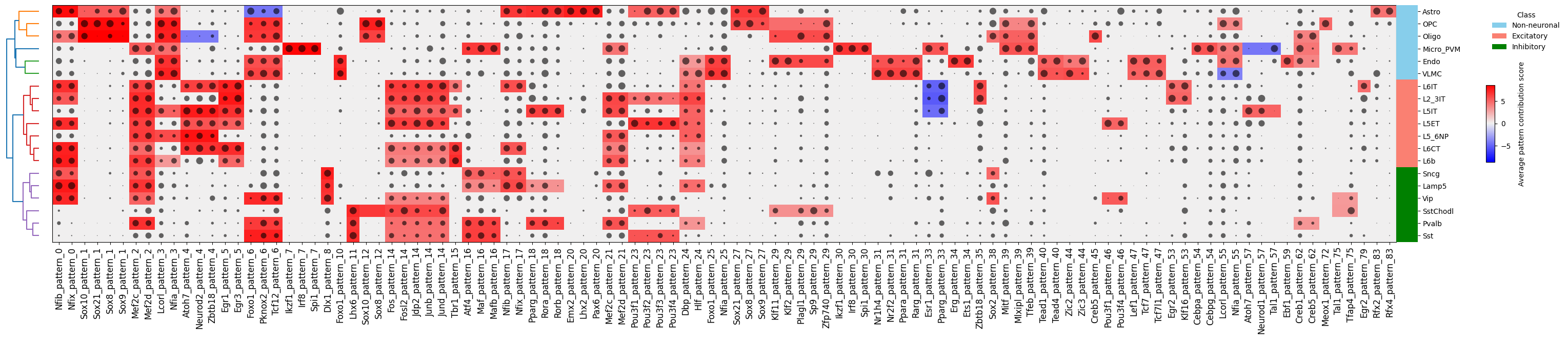
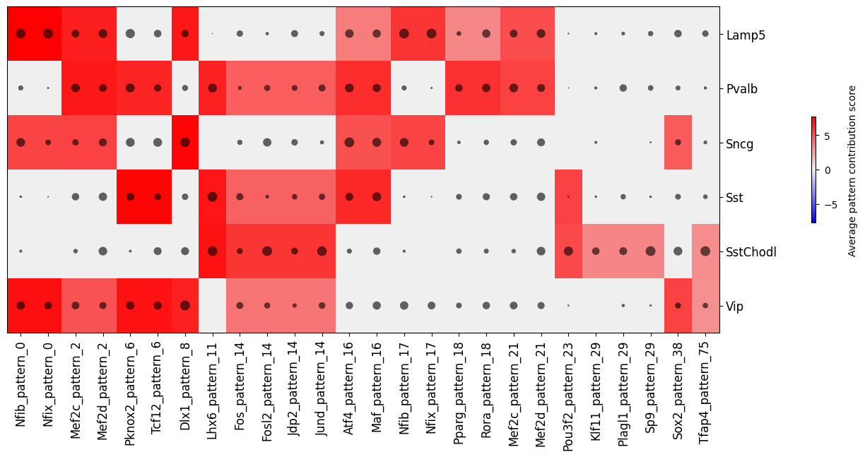
Finally, we can plot a clustermap of potential pattern-TF matches and their importance per cell type with crested.pl.modisco.clustermap_tf_motif()
# Row strip: each cell type -> coarse group (rows are class_labels, NOT pattern_ids)
def _ct_group(ct):
    if ct in nn:  return "Non-neuronal"
    if ct in exc: return "Excitatory"
    if ct in inh: return "Inhibitory"
    raise ValueError(f"Unknown class: {ct}")

row_class_mapping = {ct: _ct_group(ct) for ct in classes}
row_class_palette = {"Non-neuronal": "skyblue", "Excitatory": "salmon", "Inhibitory": "green"}  # reuse your group_colors

crested.pl.modisco.clustermap_tf_motif(
    tf_ct_matrix,
    heatmap_dim="contrib",
    dot_dim="gex",
    class_labels=classes,
    pattern_labels=tf_pattern_annots,
    width=35,
    height=6,
    cluster_rows=True,
    cluster_columns=False,
    xtick_rotation=90,
    row_class_mapping=row_class_mapping,   # cell-type -> group color strip on the row edge
    row_class_palette=row_class_palette,
    row_class_legend=True,
)
crested.pl.modisco.clustermap_tf_motif(
    tf_ct_matrix,
    heatmap_dim="contrib",
    dot_dim="gex",
    class_labels=classes,
    subset_classes=["Lamp5", "Sncg", "Vip", "Pvalb", "Sst", "SstChodl"],
    pattern_labels=tf_pattern_annots,
    width=13,
    height=6,
    cluster_rows=False,
    cluster_columns=False,
    xtick_rotation=90,
    cbar_pad=0.1
)
crested.pl.modisco.clustermap_tf_motif(
    tf_ct_matrix,
    heatmap_dim="contrib",
    dot_dim="gex",
    class_labels=classes,
    subset_classes=["L2_3IT","L5IT","L6IT","L5ET","L5_6NP","L6b","L6CT"],
    pattern_labels=tf_pattern_annots,
    width=15,
    height=6,
    cluster_rows=False,
    cluster_columns=False,
    xtick_rotation=90,
    cbar_pad=0.1
)